Matching and inverse probability weighting
Video walk-through
If you want to follow along with this example, you can download the data below:
There’s a set of videos that walks through each section below. To make it easier for you to jump around the video examples, I cut the long video into smaller pieces and included them all in one YouTube playlist.
- Drawing a DAG
- Creating an RStudio project
- Naive (and wrong!) estimate
- Matching
- Inverse probability weighting
You can also watch the playlist (and skip around to different sections) here:
Program background
Let’s revisit the mosquito net program we used in the DAG example. Here, researchers are interested in whether using mosquito nets decreases an individual’s risk of contracting malaria. They have collected data from 1,752 households in an unnamed country and have variables related to environmental factors, individual health, and household characteristics. The data is not experimental—researchers have no control over who uses mosquito nets, and individual households make their own choices over whether to apply for free nets or buy their own nets, as well as whether they use the nets if they have them.
The CSV file contains the following columns:
- Malaria risk (
malaria_risk): The likelihood that someone in the household will be infected with malaria. Measured on a scale of 0–100, with higher values indicating higher risk. - Mosquito net (
netandnet_num): A binary variable indicating if the household used mosquito nets. - Eligible for program (
eligible): A binary variable indicating if the household is eligible for the free net program. - Income (
income): The household’s monthly income, in US dollars. - Nighttime temperatures (
temperature): The average temperature at night, in Celsius. - Health (
health): Self-reported healthiness in the household. Measured on a scale of 0–100, with higher values indicating better health. - Number in household (
household): Number of people living in the household. - Insecticide resistance (
resistance): Some strains of mosquitoes are more resistant to insecticide and thus pose a higher risk of infecting people with malaria. This is measured on a scale of 0–100, with higher values indicating higher resistance.
Our goal
Our goal in this example is to estimate the causal effect of bed net usage on malaria risk using only observational data. This was not an RCT, so it might seem a little sketchy to make claims of causality. But if we can draw a correct DAG and adjust for the correct nodes, we can isolate the net → malaria relationship and talk about causality.
Because this is simulated data, we know the true causal effect of the net program because I built it into the data. The true average treatment effect (ATE) is -10. Using a mosquito net causes the risk of malaria to decrease by 10 points, on average.
Let’s see if we can find that 10 point effect!
Load data and libraries
First, let’s download the dataset (if you haven’t already), put in a folder named data, and load it:
library(tidyverse)  # ggplot(), %>%, mutate(), and friends
library(ggdag)  # Make DAGs
library(dagitty)  # Do DAG logic with R
library(broom)  # Convert models to data frames
library(MatchIt)  # Match things
library(modelsummary)  # Make side-by-side regression tables

set.seed(1234)   # Make all random draws reproducible
# Load the data.
# It'd be a good idea to click on the "nets" object in the Environment panel in
# RStudio to see what the data looks like after you load it
nets <- read_csv("data/mosquito_nets.csv")
DAG and adjustment sets
Before running any models, we need to find what we need to adjust for. Recall from the DAG example that we built this causal model to show the data generating process behind the relationship between mosquito net usage and malaria risk:
mosquito_dag <- dagify(
  malaria_risk ~ net + income + health + temperature + resistance,
  net ~ income + health + temperature + eligible + household,
  eligible ~ income + household,
  health ~ income,
  exposure = "net",
  outcome = "malaria_risk",
  coords = list(x = c(malaria_risk = 7, net = 3, income = 4, health = 5,
                      temperature = 6, resistance = 8.5, eligible = 2, household = 1),
                y = c(malaria_risk = 2, net = 2, income = 3, health = 1,
                      temperature = 3, resistance = 2, eligible = 3, household = 2)),
  labels = c(malaria_risk = "Risk of malaria", net = "Mosquito net", income = "Income",
             health = "Health", temperature = "Nighttime temperatures",
             resistance = "Insecticide resistance",
             eligible = "Eligible for program", household = "Number in household")
)

ggdag_status(mosquito_dag, use_labels = "label", text = FALSE) +
  guides(fill = FALSE, color = FALSE) +  # Disable the legend
  theme_dag()
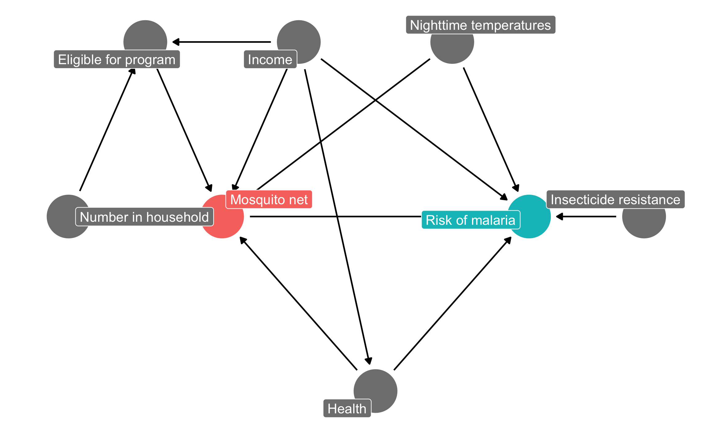
Following the logic of do-calculus, we can find all the nodes that confound the relationship between net usage and malaria risk, since those nodes open up backdoor paths and distort the causal effect we care about. We can either do this graphically by looking for any node that points to both net and malaria risk, or we can use R:
adjustmentSets(mosquito_dag)
## { health, income, temperature }
Based on the relationships between all the nodes in the DAG, adjusting for health, income, and temperature is enough to close all backdoors and identify the relationship between net use and malaria risk.
Naive correlation-isn’t-causation estimate
For fun, we can calculate the difference in average malaria risk for those who did/didn’t use mosquito nets. This is most definitely not the actual causal effect—this is the “correlation is not causation” effect that doesn’t account for any of the backdoors in the DAG.
We can do this with a table (but then we have to do manual math to subtract the FALSE average from the TRUE average):
nets %>%
  group_by(net) %>%
  summarize(number = n(),
            avg = mean(malaria_risk))
## # A tibble: 2 x 3
##   net   number   avg
##   <lgl>  <int> <dbl>
## 1 FALSE   1071  41.9
## 2 TRUE     681  25.6
Or we can do it with regression:
model_wrong <- lm(malaria_risk ~ net, data = nets)

tidy(model_wrong)
## # A tibble: 2 x 5
##   term        estimate std.error statistic   p.value
##   <chr>          <dbl>     <dbl>     <dbl>     <dbl>
## 1 (Intercept)     41.9     0.405     104.  0.
## 2 netTRUE        -16.3     0.649     -25.1 2.25e-119
According to this estimate, using a mosquito net is associated with a 16.33 point decrease in malaria risk, on average. We can’t legally talk about this as a causal effect though—there are confounding variables to deal with.
Matching
We can use matching techniques to pair up similar observations and make the unconfoundedness assumption—that if we see two observations that are pretty much identical, and one used a net and one didn’t, the choice to use a net was random.
Because we know from the DAG that income, nighttime temperatures, and health help cause both net use and malaria risk (and confound that relationship!), we’ll try to find observations with similar values of income, temperatures, and health that both used and didn’t use nets.
We can use the matchit() function from the MatchIt R package to match points based on Mahalanobis distance. There are lots of other options available—see the online documentation for details.
We can include the replace = TRUE option to make it so that points that have been matched already can be matched again (that is, we’re not forcing a one-to-one matching; we have one-to-many matching instead).
Step 1: Preprocess
matched_data <- matchit(net ~ income + temperature + health,
                        data = nets,
                        method = "nearest",
                        distance = "mahalanobis",
                        replace = TRUE)
summary(matched_data)
##
## Call:
## matchit(formula = net ~ income + temperature + health, data = nets,
##     method = "nearest", distance = "mahalanobis", replace = TRUE)
##
## Summary of Balance for All Data:
##             Means Treated Means Control Std. Mean Diff. Var. Ratio eCDF Mean eCDF Max
## income                955           873            0.41        1.4     0.104    0.198
## temperature            23            24           -0.17        1.1     0.042    0.097
## health                 55            48            0.36        1.2     0.071    0.168
##
##
## Summary of Balance for Matched Data:
##             Means Treated Means Control Std. Mean Diff. Var. Ratio eCDF Mean eCDF Max Std. Pair Dist.
## income                955           950           0.026        1.1     0.010    0.048            0.12
## temperature            23            23          -0.006        1.0     0.007    0.028            0.12
## health                 55            55           0.020        1.1     0.007    0.028            0.12
##
## Percent Balance Improvement:
##             Std. Mean Diff. Var. Ratio eCDF Mean eCDF Max
## income                   94         66        91       76
## temperature              96         61        84       71
## health                   94         61        90       83
##
## Sample Sizes:
##               Control Treated
## All              1071     681
## Matched (ESS)     323     681
## Matched           439     681
## Unmatched         632       0
## Discarded           0       0
Here we can see that all 681 of the net users were paired with similar-looking non-users (439 of them). 632 people weren’t matched and will get discarded. If you’re curious, you can see which treated rows got matched to which control rows by running matched_data$match.matrix.
We can create a new data frame of those matches with match.data():
matched_data_for_real <- match.data(matched_data)
Step 2: Estimation
Now that the data has been matched, it should work better for modeling. Also, because we used income, temperatures, and health in the matching process, we’ve adjusted for those DAG nodes and have closed those backdoors, so our model can be pretty simple here:
model_matched <- lm(malaria_risk ~ net,
                    data = matched_data_for_real)
tidy(model_matched)
## # A tibble: 2 x 5
##   term        estimate std.error statistic  p.value
##   <chr>          <dbl>     <dbl>     <dbl>    <dbl>
## 1 (Intercept)     38.5     0.600      64.2 0.
## 2 netTRUE        -12.9     0.769     -16.8 2.31e-56
The 12.88 point decrease here is better than the naive estimate, but it’s not the true 10 point causal effect (that I built in to the data). Perhaps that’s because the matches aren’t great, or maybe we threw away too much data. There are a host of diagnostics you can look at to see how well things are matched (check the documentation for MatchIt for examples.)
Actually, the most likely culprit for the incorrect estimate is that there’s some imbalance in the data. Because we set replace = TRUE, we did not do 1:1 matching—untreated observations were paired with more than one treated observation. As a result, the multiply-matched observations are getting overcounted and have too much importance in the model. Fortunately, matchit() provides us with a column called weights that allows us to scale down the overmatched observations when running the model. Importantly, these weights have nothing to do with causal inference or backdoors or inverse probability weighting—their only purpose is to help scale down the imbalance arising from overmatching. If you use replace = FALSE and enforce 1:1 matching, the whole weights column will just be 1.
We can incorporate those weights into the model and get a more accurate estimate:
model_matched_wts <- lm(malaria_risk ~ net,
                        data = matched_data_for_real,
                        weights = weights)
tidy(model_matched_wts)
## # A tibble: 2 x 5
##   term        estimate std.error statistic  p.value
##   <chr>          <dbl>     <dbl>     <dbl>    <dbl>
## 1 (Intercept)     36.1     0.595      60.6 0.
## 2 netTRUE        -10.5     0.763     -13.7 7.98e-40
After weighting to account for under- and over-matching, we find a -10.49 point causal effect. That’s much better than any of the other estimates we’ve tried so far! The reason it’s accurate is because we’ve closed the confounding backdoors and isolated the arrow between net use and malaria risk.
Inverse probability weighting
One potential downside to matching is that you generally have to throw away a sizable chunk of your data—anything that’s unmatched doesn’t get included in the final matched data.
An alternative approach to matching is to assign every observation some probability of receiving treatment, and then weight each observation by its inverse probability—observations that are predicted to get treatment and then don’t, or observations that are predicted to not get treatment and then do will receive more weight than the observations that get/don’t get treatment as predicted.
Generating these inverse probability weights requires a two step process: (1) we first generate propensity scores, or the probability of receiving treatment, and then (2) we use a special formula to convert those propensity scores into weights. Once we have inverse probability weights weights, we can incorporate them into our regression model.
Oversimplified crash course in logistic regression
There are many ways to generate propensity scores (like logistic regression, probit regression, and even machine learning techniques like random forests and neural networks), but logistic regression is probably the most common method.
The complete technical details of logistic regression are beyond the scope of this class, but if you’re curious you should check out this highly accessible tutorial.
All you really need to know is that the outcome variable in logistic regression models must be binary, and the explanatory variables you include in the model help explain the variation in the likelihood of your binary outcome. The Y (or outcome) in logistic regression is a logged ratio of probabilities, which forces the model’s output to be in a 0-1 range:
$$ \log \frac{p_y}{p_{1-y}} = \beta_0 + \beta_1 x_1 + \beta_2 x_2 + \dots + \beta_n x_n + \epsilon $$
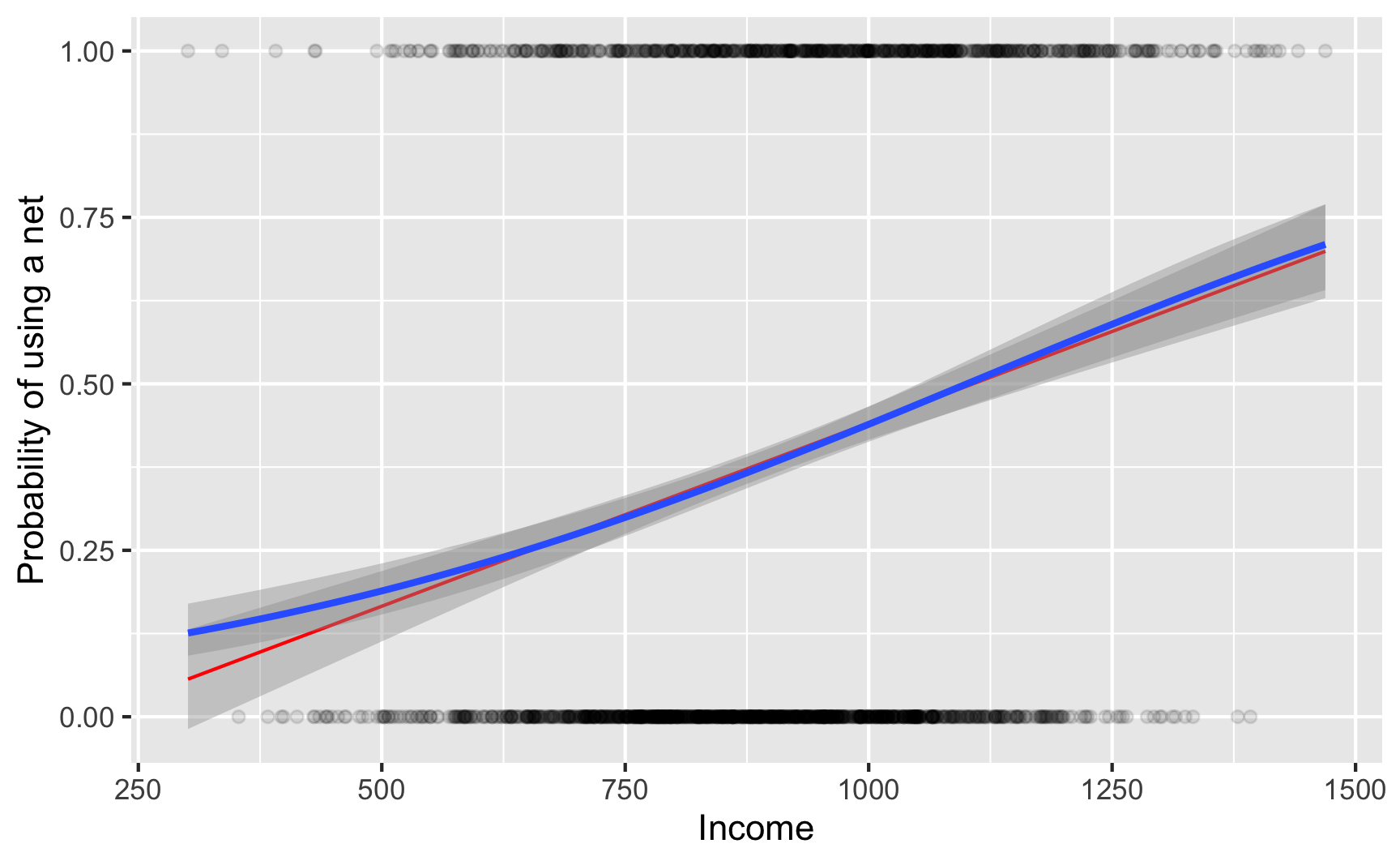
Here’s what it looks like visually. Because net usage is a binary outcome, there are lines of observations at 0 and 1 along the y axis. The blue curvy line here shows the output of a logistic regression model—people with low income have a low likelihood of using a net, while those with high income are far more likely to do so.
I also included a red line showing the results from a regular old lm() OLS model. It follows the blue line fairly well for a while, but predicts negative probabilities if you use lower values of income, like less than 250. For strange historical and mathy reasons, many economists like using OLS on binary outcomes (they even have a fancy name for it: linear probability models (LPMs)), but I’m partial to logistic regression since it doesn’t generate probabilities greater than 100% or less than 0%. (BUT DON’T EVER COMPLAIN ABOUT LPMs ONLINE. You’ll start battles between economists and other social scientists. 🤣)
ggplot(nets, aes(x = income, y = net_num)) +
  geom_point(alpha = 0.1) +
  geom_smooth(method = "lm", color = "red", size = 0.5) +
  geom_smooth(method = "glm", method.args = list(family = binomial(link = "logit"))) +
  labs(x = "Income", y = "Probability of using a net")
The coefficients from a logistic regression model are interpreted differently than you’re used to (and their interpretations can be controversial!). Here’s an example for the model in the graph above:
# Notice how we use glm() instead of lm(). The "g" stands for "generalized"
# linear model. We have to specify a family in any glm() model. You can
# technically run a regular OLS model (like you do with lm()) if you use
# glm(y ~ x1 + x2, family = gaussian(link = "identity")), but people rarely do that.
#
# To use logistic regression, you have to specify a binomial/logit family like so:
# family = binomial(link = "logit")
model_logit <- glm(net ~ income + temperature + health,
                   data = nets,
                   family = binomial(link = "logit"))

tidy(model_logit)
## # A tibble: 4 x 5
##   term        estimate std.error statistic     p.value
##   <chr>          <dbl>     <dbl>     <dbl>       <dbl>
## 1 (Intercept) -1.32     0.376        -3.50 0.000464
## 2 income       0.00209  0.000421      4.95 0.000000727
## 3 temperature -0.0589   0.0125       -4.70 0.00000264
## 4 health       0.00688  0.00430       1.60 0.109
The coefficients here aren’t normal numbers—they’re called “log odds” and represent the change in the logged odds as you move explanatory variables up. For instance, here the logged odds of using a net increase by 0.00688 for every one point increase in your health score. But what do logged odds even mean?! Nobody knows.
You can make these coefficients slightly more interpretable by unlogging them and creating something called an “odds ratio.” These coefficients were logged with a natural log, so you unlog them by raising \(e\) to the power of the coefficient. The odds ratio for temperature is \(e^{-0.0589}\), or 0.94. Odds ratios get interpreted a little differently than regular model coefficients. Odds ratios are all centered around 1—values above 1 mean that there’s an increase in the likelihood of the outcome, while values below 1 mean that there’s a decrease in the likelihood of the outcome.
Our nighttime temperature odds ratio here is 0.94, which is 0.06 below 1, which means we can say that for every one point increase in nighttime temperatures, a person is 6% less likely to use a net. If the coefficient was something like 1.34, we could say that they’d be 34% more likely to use a net; if it was something like 5.02 we could say that they’d be 5 times more likely to use a net; if it was something like 0.1, we could say that they’re 90% less likely to use a net.
You can make R exponentiate the coefficients automatically by including exponentiate = TRUE in tidy():
tidy(model_logit, exponentiate = TRUE)
## # A tibble: 4 x 5
##   term        estimate std.error statistic     p.value
##   <chr>          <dbl>     <dbl>     <dbl>       <dbl>
## 1 (Intercept)    0.268  0.376        -3.50 0.000464
## 2 income         1.00   0.000421      4.95 0.000000727
## 3 temperature    0.943  0.0125       -4.70 0.00000264
## 4 health         1.01   0.00430       1.60 0.109
BUT AGAIN this goes beyond the scope of this class! Just know that when you build a logistic regression model, you’re using explanatory variables to predict the probability of an outcome.
Just one last little explanation for why we have to use weird log odds things. When working with binary outcomes, we’re dealing with probabilities, and we can create something called “odds” with probabilities. If there’s a 70% chance of something happening, there’s a 30% chance of it not happening. The ratio of those two probabilities is called “odds”: \(\frac{p}{1 - p} = \frac{0.7}{1 - 0.7} = \frac{0.7}{0.3} = 2.333\). Odds typically follow a curvy relationship—as you move up to higher levels of your explanatory variable, the odds get bigger faster. If you log these odds, though ($\log \frac{p}{1 - p}$), the relationship becomes linear, which means we can use regular old linear regression on probabilities. Magic!
You can see the relationship between log odds and odds ratios in the first two panels here (this is fake data where X ranges between -5 and 5, and Y is either 0 or 1; you can see the data points in the final panel as dots):
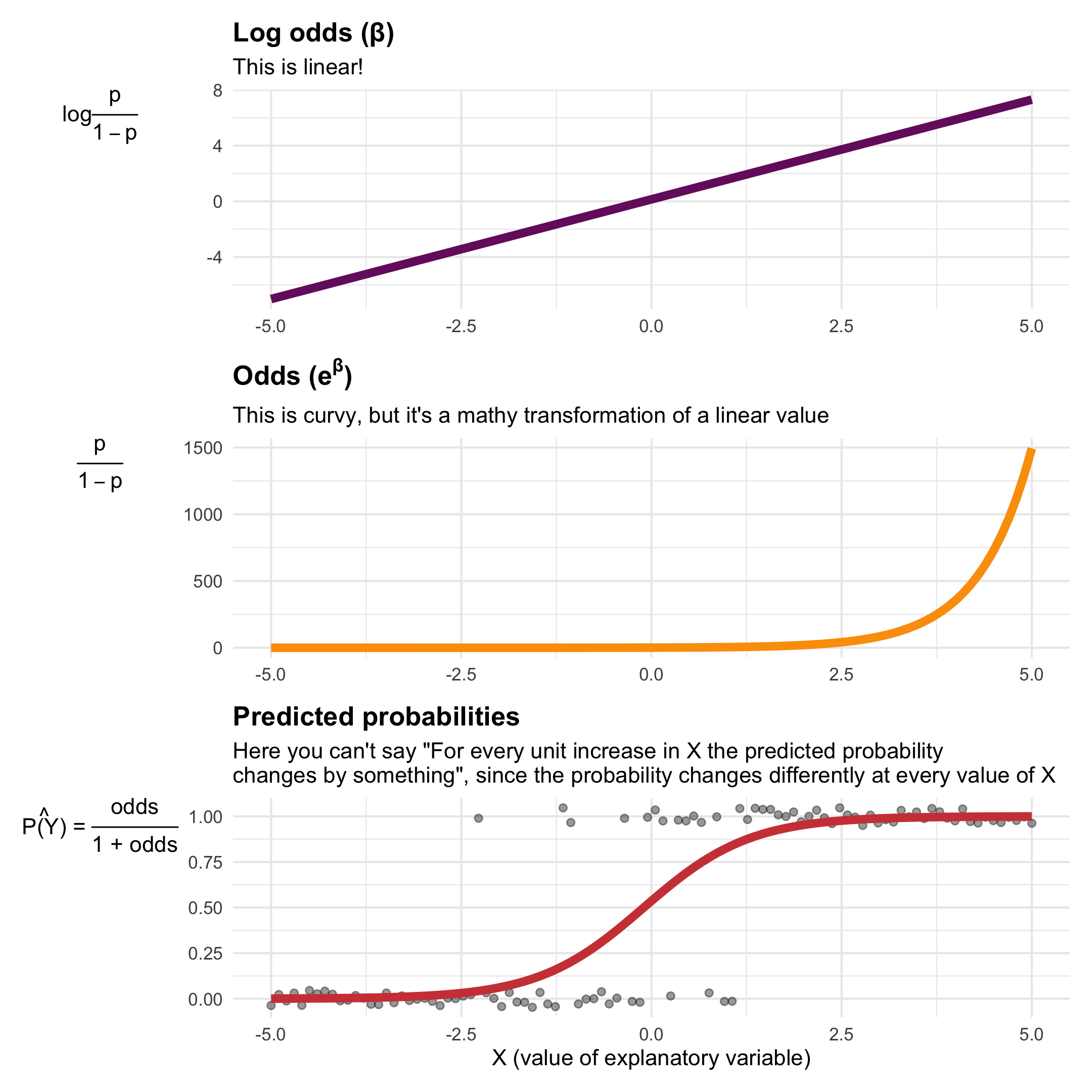
The coefficients from logistic regression are log odds because they come from model that creates that nice straight line in the first panel. Log odds are impossible to interpret, so we can unlog them ($e^\beta$) to turn them into odds ratios.
The bottom panel shows predicted probabilities. You can do one more mathematical transformation with the odds ($\frac{p}{1 - p}$) to generate a probability instead of odds: \(\frac{\text{odds}}{1 + \text{odds}}\). That is what a propensity score is.
BUT AGAIN I cannot stress enough how much you don’t need to worry about the inner mechanics of logistic regression for this class! If that went over your head, don’t worry! All we’re doing for IPW is using logistic regression to create propensity scores, and the code below shows how to do that. Behind the scenes you’re moving from log odds (they’re linear!) to odds (they’re interpretable-ish) to probabilities (they’re super interpretable!), but you don’t need to worry about that.
If you’re confused, watch this TikTok for consolation.
Step 1: Generate propensity scores
PHEW. With that little tangent into logistic regression done, we can now build a model to generate propensity scores (or predicted probabilities).
When we include variables in the model that generates propensity scores, we’re making adjustments and closing backdoors in the DAG, just like we did with matching. But unlike matching, we’re not throwing any data away! We’re just making some observations more important and others less important.
First we build a model that predicts net usage based on income, nighttime temperatures, and health (since those nodes are our confounders from the DAG):
model_net <- glm(net ~ income + temperature + health,
                 data = nets,
                 family = binomial(link = "logit"))

# We could look at these results if we wanted, but we don't need to for this class
# tidy(model_net, exponentiate = TRUE)
We can then plug in the income, temperatures, and health for every row in our dataset and generate a predicted probability using this model:
# augment_columns() handles the plugging in of values. You need to feed it the
# name of the model and the name of the dataset you want to add the predictions
# to. The type.predict = "response" argument makes it so the predictions are in
# the 0-1 scale. If you don't include that, you'll get predictions in an
# uninterpretable log odds scale.
net_probabilities <- augment_columns(model_net,
                                     nets,
                                     type.predict = "response") %>%
  # The predictions are in a column named ".fitted", so we rename it here
  rename(propensity = .fitted)

# Look at the first few rows of a few columns
net_probabilities %>%
  select(id, net, income, temperature, health, propensity) %>%
  head()
## # A tibble: 6 x 6
##      id net   income temperature health propensity
##   <dbl> <lgl>  <dbl>       <dbl>  <dbl>      <dbl>
## 1     1 TRUE     781        21.1     56      0.367
## 2     2 FALSE    974        26.5     57      0.389
## 3     3 FALSE    502        25.6     15      0.158
## 4     4 TRUE     671        21.3     20      0.263
## 5     5 FALSE    728        19.2     17      0.308
## 6     6 FALSE   1050        25.3     48      0.429
The propensity scores are in the propensity column. Some people, like person 3, are unlikely to use nets (only a 15.8% chance) given their levels of income, temperature, and health. Others like person 6 have a higher probability (42.9%) since their income and health are higher. Neat.
Next we need to convert those propensity scores into inverse probability weights, which makes weird observations more important (i.e. people who had a high probability of using a net but didn’t, and vice versa). To do this, we follow this equation:
$$ \frac{\text{Treatment}}{\text{Propensity}} - \frac{1 - \text{Treatment}}{1 - \text{Propensity}} $$
This equation will create weights that provide the average treatment effect (ATE), but there are other versions that let you find the average treatment effect on the treated (ATT), average treatment effect on the controls (ATC), and a bunch of others. You can find those equations here.
We’ll use mutate() to create a column for the inverse probability weight:
net_ipw <- net_probabilities %>%
  mutate(ipw = (net_num / propensity) + ((1 - net_num) / (1 - propensity)))

# Look at the first few rows of a few columns
net_ipw %>%
  select(id, net, income, temperature, health, propensity, ipw) %>%
  head()
## # A tibble: 6 x 7
##      id net   income temperature health propensity   ipw
##   <dbl> <lgl>  <dbl>       <dbl>  <dbl>      <dbl> <dbl>
## 1     1 TRUE     781        21.1     56      0.367  2.72
## 2     2 FALSE    974        26.5     57      0.389  1.64
## 3     3 FALSE    502        25.6     15      0.158  1.19
## 4     4 TRUE     671        21.3     20      0.263  3.81
## 5     5 FALSE    728        19.2     17      0.308  1.44
## 6     6 FALSE   1050        25.3     48      0.429  1.75
These first few rows have fairly low weights—those with low probabilities of using nets didn’t, while those with high probabilities did. But look at person 4! They only had a 26% chance of using a net and they did! That’s weird! They therefore have a higher inverse probability weight (3.81).
Step 2: Estimation
Now that we’ve generated inverse probability weights based on our confounders, we can run a model to find the causal effect of mosquito net usage on malaria risk. Again, we don’t need to include income, temperatures, or health in the model since we already used them when we created the propensity scores and weights:
model_ipw <- lm(malaria_risk ~ net,
                data = net_ipw,
                weights = ipw)

tidy(model_ipw)
## # A tibble: 2 x 5
##   term        estimate std.error statistic  p.value
##   <chr>          <dbl>     <dbl>     <dbl>    <dbl>
## 1 (Intercept)     39.7     0.468      84.7 0.
## 2 netTRUE        -10.1     0.658     -15.4 3.21e-50
Cool! After using the inverse probability weights, we find a -10.13 point causal effect. That’s a tiiiny bit off from the true value of 10, but not bad at all!
It’s important to check the values of your inverse probability weights. Sometimes they can get too big, like if someone had an income of 0 and the lowest possible health and lived in a snow field and yet still used a net. Having really really high IPW values can throw off estimation. To fix this, we can truncate weights at some lower level. There’s no universal rule of thumb for a good maximum weight—I’ve often seen 10 used. In our mosquito net data, no IPWs are higher than 10 (the max is exactly 10 with person 877), so we don’t need to worry about truncation.
If you did want to truncate, you’d do something like this (here we’re truncating at 8 instead of 10 so truncation actually does something):
net_ipw <- net_ipw %>%
  # If the IPW is larger than 8, make it 8, otherwise use the current IPW
  mutate(ipw_truncated = ifelse(ipw > 8, 8, ipw))

model_ipw_truncated <- lm(malaria_risk ~ net,
                          data = net_ipw,
                          weights = ipw_truncated)

tidy(model_ipw_truncated)
## # A tibble: 2 x 5
##   term        estimate std.error statistic  p.value
##   <chr>          <dbl>     <dbl>     <dbl>    <dbl>
## 1 (Intercept)     39.7     0.467      85.1 0.
## 2 netTRUE        -10.2     0.656     -15.5 4.32e-51
Now the causal effect is -10.19, which is slightly lower and probably less accurate since we don’t really have any exceptional cases messing up our original IPW estimate.
Results from all the models
All done! We just used observational data to estimate causal effects. Causation without RCTs! Do you know how neat that is?!
Let’s compare all the ATEs that we just calculated:
modelsummary(list("Naive" = model_wrong,
                  "Matched" = model_matched, "Matched + weights" = model_matched_wts,
                  "IPW" = model_ipw, "IPW truncated at 8" = model_ipw_truncated))
| Naive | Matched | Matched + weights | IPW | IPW truncated at 8 | |
|---|---|---|---|---|---|
| (Intercept) | 41.937*** | 38.487*** | 36.094*** | 39.679*** | 39.679*** |
| (0.405) | (0.600) | (0.595) | (0.468) | (0.467) | |
| netTRUE | -16.332*** | -12.882*** | -10.489*** | -10.131*** | -10.190*** |
| (0.649) | (0.769) | (0.763) | (0.658) | (0.656) | |
| Num.Obs. | 1752 | 1120 | 1120 | 1752 | 1752 |
| R2 | 0.265 | 0.201 | 0.145 | 0.119 | 0.121 |
| R2 Adj. | 0.265 | 0.200 | 0.144 | 0.119 | 0.121 |
| AIC | 14030.7 | 8851.7 | 8890.0 | 14274.3 | 14260.5 |
| BIC | 14047.1 | 8866.8 | 8905.0 | 14290.7 | 14276.9 |
| Log.Lik. | -7012.326 | -4422.846 | -4441.978 | -7134.172 | -7127.255 |
| F | 632.315 | 280.581 | 188.862 | 236.841 | 241.379 |
| Deviance | 307298.43 | 176512.42 | 173842.84 | 668442.23 | 663098.21 |
| DF Resid | 1750 | 1118 | 1118 | 1750 | 1750 |
| Sigma | 13.251 | 12.565 | 12.470 | 19.544 | 19.466 |
| Statistics | 632.315 | 280.581 | 188.862 | 236.841 | 241.379 |
| p | 0.000 | 0.000 | 0.000 | 0.000 | 0.000 |
| DF | 1 | 1 | 1 | 1 | 1 |
| * p < 0.1, ** p < 0.05, *** p < 0.01 |
Which one is right? In this case, because this is fake simulated data where I built in a 10 point effect, we can see which of these models gets the closest: here, the non-truncated IPW model wins. But that won’t always be the case. Both matching and IPW work well for closing backdoors and adjusting for confounders. In real life, you won’t know the true value, so try multiple ways.